Experimental correlation and model updating is a critical step for model validation and thus the generation of digital twins. VibTwin has extensive expertise in this domain based on SDT capabilities and past experience. You will find on this page a brief discussion on the method, showcasing the benefits you can gain by having access to advanced correlation and updating solutions.
Traditional correlation means in vibrations
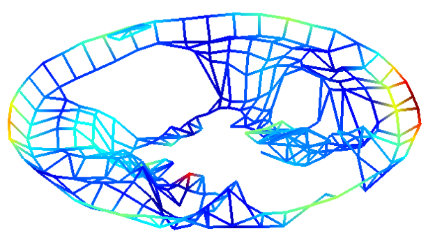
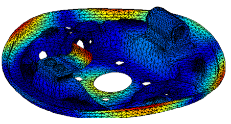
In vibrations, the Experimental Modal Analysis (EMA) technique identifies modeshapes associated with frequencies and damping using Frequency Response Functions (FRF) fitting algorithms. One thus typically starts correlation with a series of experimental and numerical modeshapes such as the ones illustrated for a drum brake backplate below.
The Modal Assurance Criterion (MAC) as a starting point
Frequency and shape errors are then measured. The proper procedures require fitting the test mesh on the model to generate an observation matrix in order to obtain the expression of the numerical modeshapes on the test mesh.
Shape comparison comes next, with the Modal Assurance Criterion (MAC) defined by
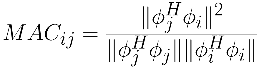
Despite not being a metric stricto-sensu, this indicator has become the easiest and most widespread way of comparing shapes. The shape-paired modes can then also be compared in terms of frequency and possibly damping. Directly comparing frequencies without paring induces the assumption that modal order obtained from the model is correct. It is often not the case due to mode crossing, quasi-multiples or lack of initial correlation in realistic applications.
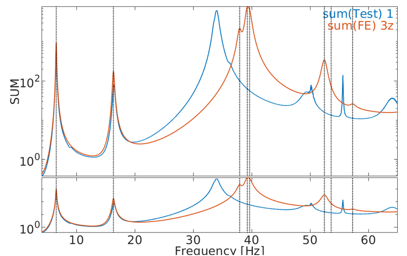
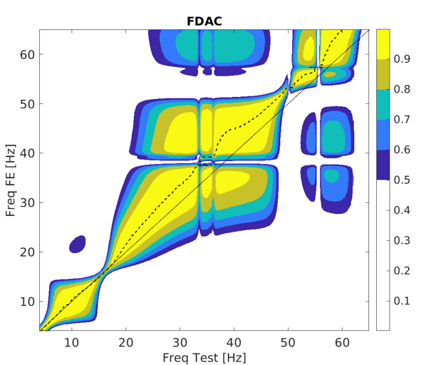
FDAC checks, the MAC for FRF
Without having direct access to experimental modal analysis, it is also possible to compare FRF directly with the FDAC, the MAC equivalent to treat FRF. Frequency pairing visualization can help in some cases. Subspace methods are nevertheless required to do a proper characterization that can be exploited for advanced correlation.
MACCo: Error localization with the MAC
In case of poor MAC results, a directly accessible method to localize discrepancies is the MACCo. It consists in sequentially removing sensors best improving target MAC values. If removed sensors are common to several modes, or induce great variations, correlation errors can be directly assessed. Sensor or model quality in the located region is subsequently investigated.
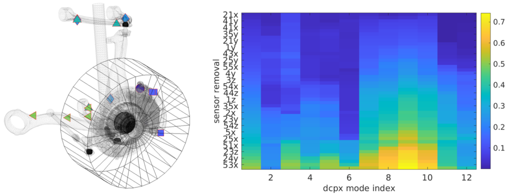
The following MACCo example shows a corner brake squeal correlation problem (low MAC values between the experimental shape and all system modes).
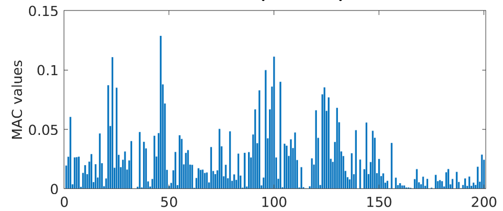
The MACCo can rank the sensors, highlighted with colors, the cooler the color the earlier it was removed. In this case, the bracket was prioritized.
Notions of subspace and mode crossing
The MAC and derivatives have many intrinsic limitations (discussed by Allemang, its inventor himself) that prevents correlation progress in project and companies not having access to more advanced solutions. MAC results can even be misleading in some cases, with projects focusing on poor MAC values without actually bad correlation.
Matching several coupled modes: subspace projection
Model perfection and physical realization
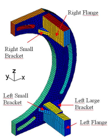
A typical example is mode crossing patterns. Consider a fully symmetrical CAO based model and an imperfect realization with a small symmetry default. The multiple mode from symmetry may not be realized resulting in poor MAC results, which does not mean that the base model is far. Let’s take a simple bracket example with two symmetrical columns, and let’s vary the height of the left column only by a small margin.
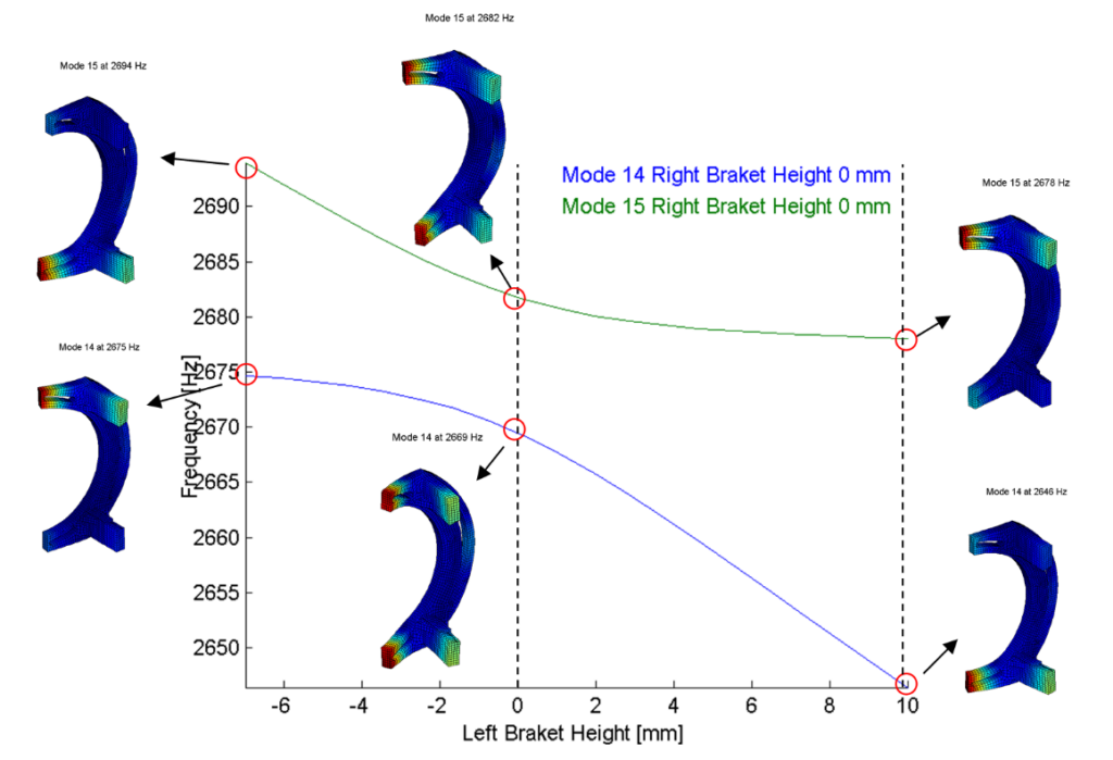
The first column bending mode is supposedly a double mode. If the columns are not perfectly symmetrical, both bending modes are decoupled and two different shapes occur.
Subspace projection concept
The right way of comparing these modes is to consider both modes at once. This solution is not MAC compatible as it is only shape-to-shape. Considering both modes implies that the subspace spanned by the modes is considered. Comparisons must then be performed with a metric able to define a distance measure from subspace projection.
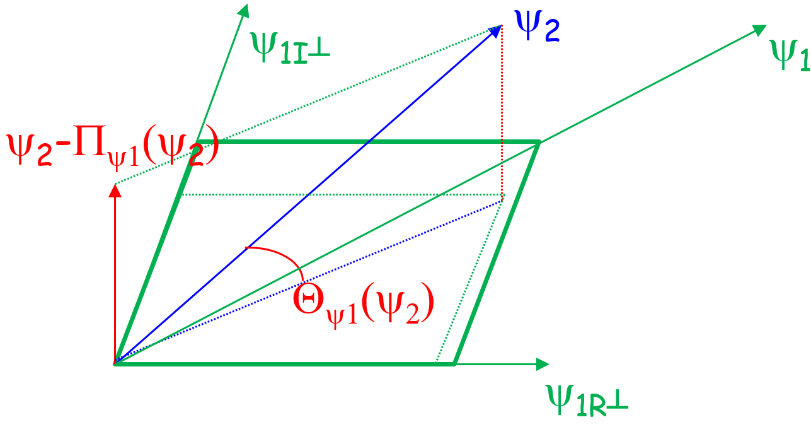
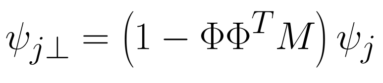
Projection of a shape into a subspace is a direct operation:
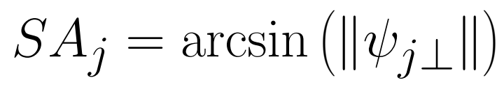
The distance can then be evaluated as the angle between subspaces;
MAC recombination to qualify coupled modes correlation
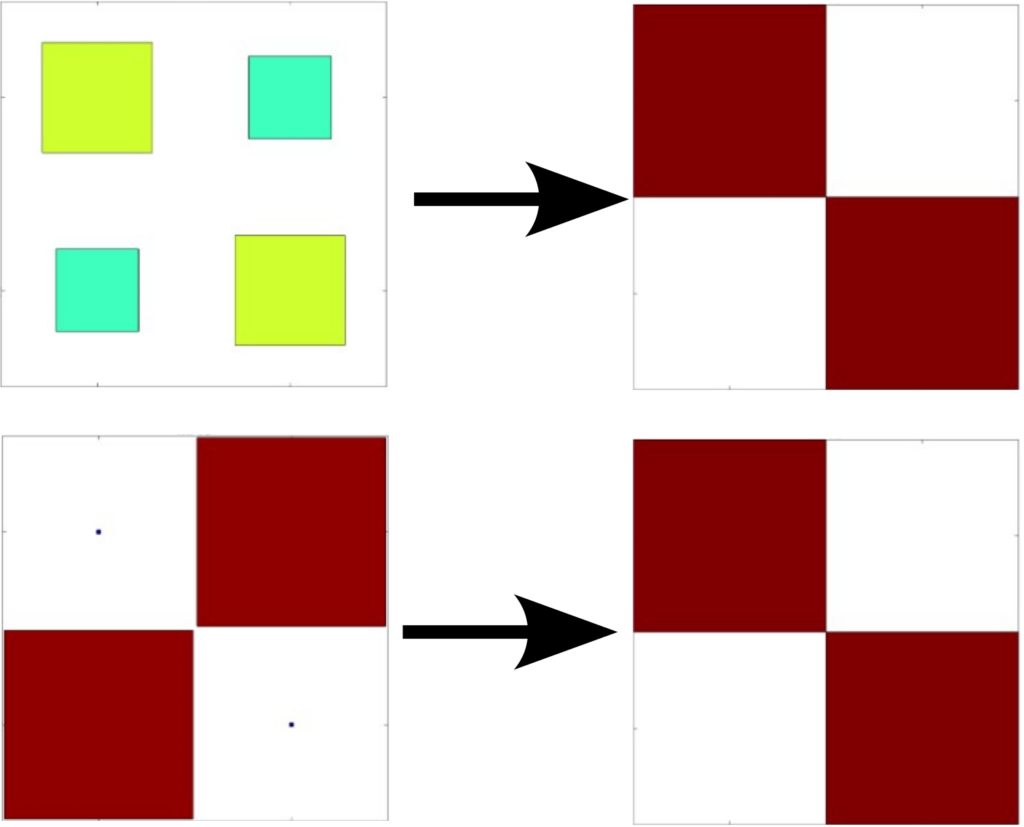
Eventually the projection method allows finding the best combination of the second subspace shapes to match the directions of the first one. For our bracket example, one recovers a clean MAC with this subspace method in every case. For the illustration below, the top recombination is obtained between the double mode setup and an asymmetrical version that resulted in an overall poor MAC.
On the second example, order was inverted between two very close asymmetrical configurations. In both cases, a good correlation exists and should be presented as such with a diagonal MAC. Do not forget the frequency and damping errors to finalize validation!
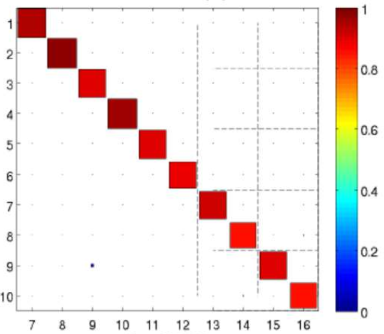
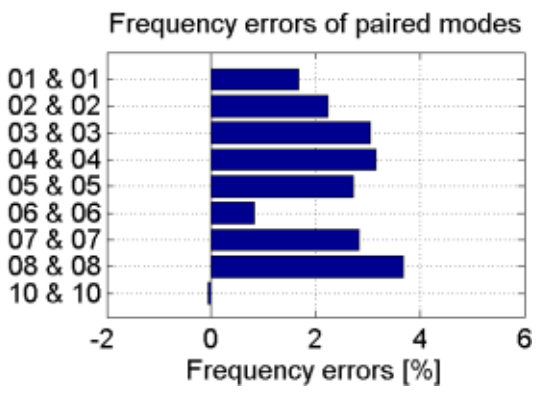
When the subspaces do not fully match
For the multiple mode matching case, one expects an all-or-nothing behavior. When increasing complexity, either when looking at higher frequencies or multi-component assemblies, partial discrepancies can happen. The example below considers a drum brake backplate for which modes 7 and 8 are very close in frequency while remaining different due to their interaction with the fitted equipment. The initial MAC is poor for both, recombination using subspace projection is performed due to the close frequency values.
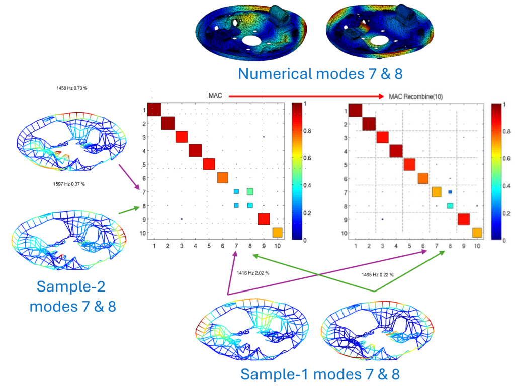
The recombined result here was very interesting and allowed critical progress. Only one direction was common, and the second mode only was poorly correlated. Further analysis using this insight helped localizing discrepancy to the equipment connection.
Expansion methods for advanced correlation
Expansion to observe test results on the model
Base correlation methods consider the test as an absolute reference, and work with the test mesh. It induces limitations, since test errors can also happen. Besides, experimental test meshes are coarse and partial by nature, preventing advanced mechanical analysis.
The expansion method allows estimating a full finite element field compatible with the test observation. Let’s take the example of an engine cradle first torsion mode:
The test shape is coarse despite the number of used accelerometers; the expansion objective is then to estimate the best test observation fitting mechanical deformation. This is an ill-posed problem solved by an inverse method. The basic idea is to use the current although imperfect model to regularize the solution.
Several techniques exist. The simplest static expansion, for example, considers a static uplift from the sensor displacement constraint applied to the mesh as if is was a Guyan interface to the real world.
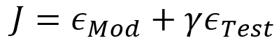
Advanced methods exist with better performance considering a quadratic functional weighting test error and model error. The Minimum Dynamic Residue Expansion (MDRE) method implemented in SDT uses a factor on the test side
The test error is chosen as the Euclidean distance at sensor positions, and the model error is expressed as a displacement field resulting from residue forces. These forces describe the discrepancy from the equilibrium state assumed on the model side. Their expression and illustrated meaning are shown below
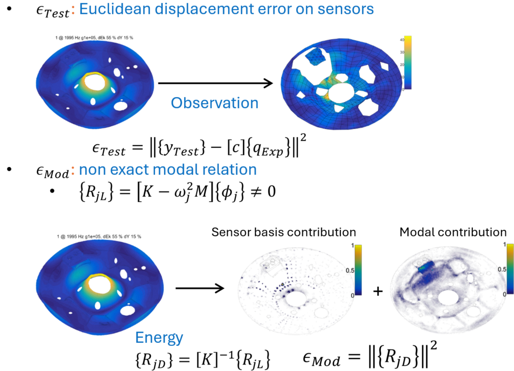
Using modal reduction and an augmented state for sensor displacements, one is able to distinguish the optimal estimation the contribution of system modes and sensor modes.
Error metric and localization
The initial objective of expansion techniques is to enable visualizing measured test fields. The resolution techniques can provide much more insight. Indeed, using dynamic residue provides an error field expressed as a displacement of the finite element model. Going further it becomes possible to compute local strain energy densities and localize model discrepancies. Moreover, splitting sensor and modal energy contributions allow assessing local distortions induced by experimental noise from model sources.
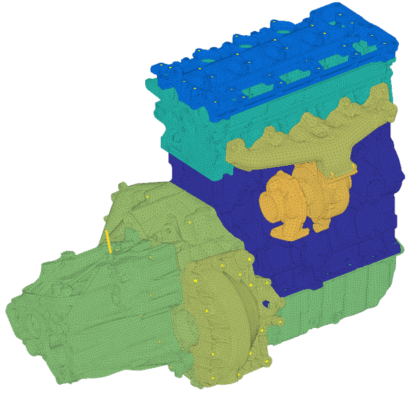
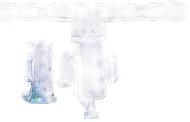
The two following examples show how model error can be used to localize discrepancies. On a full powertrain with initially significant frequency discrepancies, a precise localization on the turbo part could be obtained.
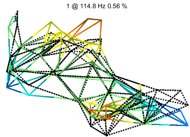
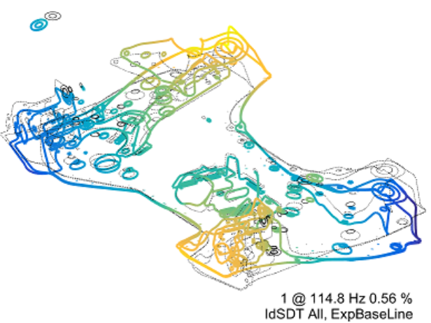
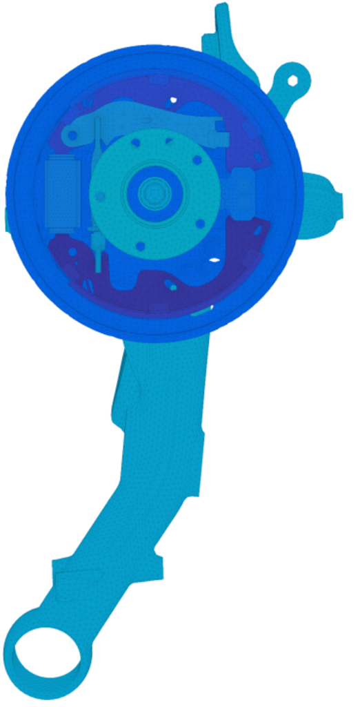
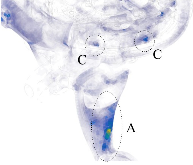
On this drum brake example, a coarse accelerometer mesh was set for a noise problem. The Expansion technique allowed obtaining a refined estimation of the deflection shape associated with the noise. The error field gave further model error indications for updating.
Expansion optimization: towards model updating
With an error metric, it is easier to set up optimization algorithms. Setting a model error minimization linked to a set of parameters becomes possible to provide updated models or constitutive law parameters identification.
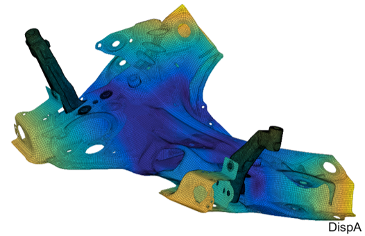
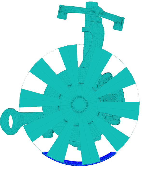
In the squeal example below, the noise was only occurring on the road. We fitted the model with a complete wheel (simplified display for publication) and had no direct clue about the wheel tire support stiffness that was sensitive. Using the expansion error metric, we obtained an accurate tuning factor for the tire support value.
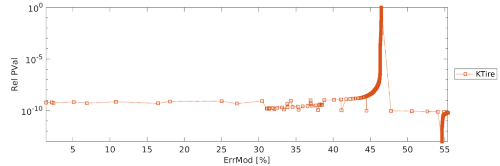
This example features a 4.4 Milion DOF system. 100 modes were computed for a 500 points logarithmic tire support stiffness factor variation between 10-12 and 1. The reduction basis took 1 hour, expansion and optimization an additional 15 minutes.